Wize University Statistics Textbook > Sampling Distribution

Sampling Distribution for a Mean

Central Limit Theorem (CLT)

The Central Limit Theorem (CLT) describes the relationship between the sampling distribution of sample means and the population that the samples are drawn from.

Suppose you are drawing samples of size $n$ from a population of size $N$ , which has mean $\mu$ and standard deviation $\sigma$ .

The CLT basically says that "for large sample sizes, the sampling distribution of any sample mean becomes close to a normal distribution."

Image illustrating Central Limit Theorem

What Does the CLT Formally Tell Us?

If the following conditions are met:

the samples are randomly drawn from the population (SRS), and
the sample size $\bm{\purple n}$ is sufficiently large (some textbooks say $n\ge25$ some say $n\ge 30$ )

then, the CLT tells us two things:

If the population is normally distributed, then the sampling distribution of the sample mean $\bar{x}$ is exactly normal.

If the population is NOT normally distributed, then the sampling distribution of the sample mean $\bar{x}$ will be approximately normal. Note: As you increase the sample size, the shape of the sampling distribution will look more and more normal.

Mean & Standard Deviation of the Sample Mean

If $n$ is large enough ( $n\ge25$ ), then the CLT tells us that the sampling distribution of the sample mean is approximately normal.

So, we have the following two properties:

The mean of the sample mean = population mean

\boxed{\mu_{\bar{x}}=\mu}

The standard deviation of the sample mean = population standard deviation divided by the square root of $n$

\boxed{\sigma_{\overline{x}}=\frac{\sigma}{\sqrt{n}}}

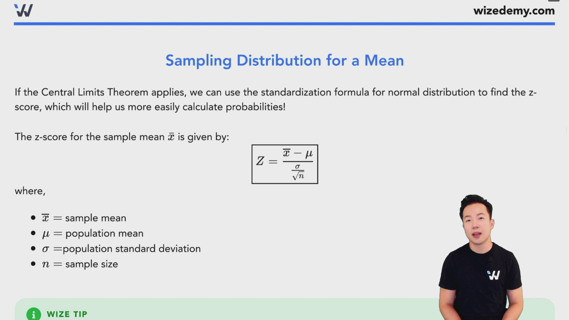
Sampling Distribution for a Mean

If the Central Limits Theorem applies, we can use the standardization formula for normal distribution to find the z-score, which will help us more easily calculate probabilities!

The z-score for the sample mean $\bar{x}$ is given by:

$\displaystyle \boxed{Z=\frac{\overline{x}-\mu}{\frac{\sigma}{\sqrt{n}}}}$

where,

$\overline{x}=$ sample mean
$\mu=$ population mean
$\sigma=$ population standard deviation
$n=$ sample size

Example: Sampling Distribution for a Mean

Random bags of potatoes weigh on average 10 pounds and have a variance of 0.64.

$\mu$ = 10, $\sigma= \sqrt{0.64}$ = 0.80

1. If you randomly select a bag of potatoes, what is the probability that it will weigh more than 8.2 pounds?

The question is asking about a single observation, let's use the $\boxed{\displaystyle z=\frac{x-\mu}{\sigma}}$ formula.

$\displaystyle z=\frac{8.2-10}{\sqrt{0.64}}=\frac{8.2-10}{0.8}=-2.25$

Using the z-table, we get $P(z<-2.25)=0.0122$

Therefore,

$P(X>8.2)$

$=P(Z>-2.25)$

$=1-0.0122$

$=0.9878$

2. If you randomly select 25 bags of potatoes, what is the probability that their average weight will be between 9.7 and 10.4 pounds?

The question is asking about the mean (average) of a sample, let's use the $\boxed{\displaystyle z= \frac{\bar{x}-\mu}{\frac{\sigma}{\sqrt{n}}}}$ formula.

$\displaystyle z= \frac{9.7-10}{\frac{0.80}{\sqrt{25}}}=-1.88$

Using the z-table, we get $P(Z<-1.88)=0.0301$

$\displaystyle z= \frac{10.4-10}{\frac{0.80}{\sqrt{25}}}=2.50$

Using the z-table, we get $P(Z<2.50)=0.9938$

Therefore,

$P(9.7<\overline{x}<10.4)$

$=P(-1.88<Z<2.50)$

$=0.9938-0.0301$

$=0.9637$

Note: Some courses require $\ge30$ for CLT to hold. If this is required in your class, then a sample size of 25 is not enough. You can still do this question for practice.

3. If you randomly select 81 bags of potatoes, what is the probability that their total weight will be at least 828 pounds?

A total weight of at least 828 means that their average is at least $\displaystyle {\bar{x}=\frac{828}{81}\approx10.222}$ .

The question is asking about the mean (average) of a sample, let's use the $\boxed{\displaystyle z= \frac{\bar{x}-\mu}{\frac{\sigma}{\sqrt{n}}}}$ formula.

$\displaystyle z= \frac{10.222-10}{\frac{0.8}{\sqrt{81}}}=2.50$

Using the z-table, we get $P(Z<2.50)=0.9938$

Therefore,

$P(\overline{x}\ge10.222)\$

$=P(Z>2.50)$

$=1-0.9938$

$=0.0062$

4. If you randomly select 10 potatoes, is there enough info to find the probability that their average is under 9.5 pounds?

Since $n$ < 25, Central Limit Theorem doesn't apply, we need a normal population to proceed. Since we don’t have that information we can’t proceed to answer this question.

Extra Practice

Sampling Distribution

True or false?

If the sample size is large enough, then the sampling distribution of X will be approximately normal, even if the population distribution is quite skewed.

Statistical sampling

Poke Mania can sell an average of 90 poke bowls a day with a standard deviation 7.18; however, the sales are not normally distributed. In fact, the distribution of sales is skewed to the right. Which of the following is true about the sampling distribution of 50 days?

Sampling Distribution for a Mean

Twin Pines Diner makes mediocre CLT (cabbage, leeks, and turnip) sandwiches. Suppose the average amount of sodium of all CLT sandwiches is 650mg, and the distribution is skewed to the right. If someone randomly samples 200 CLT sandwiches, which of the following is true?

Sampling Distribution for a Mean

The population distribution is skewed to the right. The sample size is 1000. The 95% confidence interval is [$800, $1,200].

True or false: The sample mean must be $1,000.

Sampling Distribution for a Mean Question

Sony is interested in the number of songs on a person’s iPhone. The population distribution of songs is normal with a mean of 300 and a standard deviation of 60.

(a) What’s the probability that a random iPhone will have more than 375 songs?

(b) If Sony randomly samples 12 iPhones, what’s the probability that the sample mean will be more than 375 songs?

Sampling Distribution for a Mean

Suppose that we look at the height of students at ABC University and know their average height is $\mu=160 \space\text{cm}$ and vary according to a standard deviation $\sigma=10 \space \text{cm}$ . What are the mean and standard deviation of the sampling distribution of the sample mean with n = 30 observations?

Sampling Distribution for a Mean

Kick the Butt is interested in the number of cigarettes on a smoker smokes a day. The distribution number of cigarettes is normal with a mean of 15 and a standard deviation of 8.

1. What’s the probability that a random smoker smokes more than 20 cigarettes a day?

2. If they randomly sample 10 smokers, what’s the probability that the sample mean will be more than 13 cigarettes a day?

Sampling Distribution for a Mean

The Pogs Fan Club only has 150 members. The number of pogs a member owns is normally distributed with a mean of 265 and standard deviation of 35. What is the probability of selecting a random sample of 10 members with a sample mean of 280 or more?

Sampling Distribution for a Mean

Suppose that the mean height of 10 year old males is 138.4 cm with a standard deviation of 9.6 cm. From 30 randomly selected 10 year old males, what is the probability the sample mean is greater than 140 cm?

Sampling Distribution for a Mean

Suppose that the mean height of 5 year old females is 107.9 cm with a standard deviation of 11.1 cm. If height is normally distributed, and you consider a random sample of 10 girls, then the sampling distribution for the corresponding sample mean

Sampling Distribution for a Mean

Suppose that we look at the height of students at ABC University and know their average height is $\mu=160 \space\text{cm}$ and vary according to the standard deviation $\sigma=10 \space \text{cm}$

What are the mean and standard deviation of the sampling distribution of the sample mean with n = 30 observations?

Sampling Distribution for a Mean

Suppose that you have a population that's skewed to the left.

You wish to plot the sampling distribution of the sample mean for

all samples of 40 observations.

Sampling distribution for a mean

Which of the following statements best describes the Central Limit Theorem?

Sampling Distribution for a Mean

In a certain city, the income level of its residents follow the normal model with mean $40,000 and standard deviation $18,000. A resident is considered wealthy if he/she earns more than $60,000.

A random sample of 400 residents is drawn from this city. Find the probability that more than 15% of them are wealthy.

Sampling Distribution for a Mean

Sampling Distribution for a Mean Question

Sony is interested in the number of songs on a person’s iPhone. The population distribution of songs is normal with a mean of 300 and a standard deviation of 60.

(a) What’s the probability that a random iPhone will have more than 375 songs?

(b) If Sony randomly samples 12 iPhones, what’s the probability that the sample mean will be more than 375 songs?

Sampling Distribution for a Mean

Sampling Distribution for a Mean

Create a free account to get started

Central Limit Theorem (CLT)

What Does the CLT Formally Tell Us?

Mean & Standard Deviation of the Sample Mean

Create a free account to get started

Sampling Distribution for a Mean

Create a free account to get started

Example: Sampling Distribution for a Mean

Create a free account to get started

Extra Practice