Wize AP Statistics Textbook > Linear Regression
Solving for the Regression Line

0:00 / 0:00
Solving for the Regression Line (r, Sy, Sx Method)

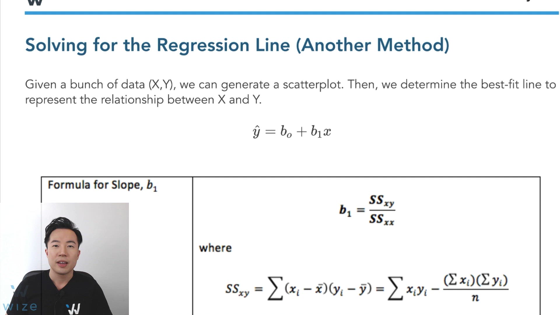
Given a bunch of data coordinates (X,Y), we can generate a scatterplot. Then, we determine the best-fit line to represent the relationship between two quantitative variables: the explanatory variable and the response variable .
The slope , tells us how much changes for every one unit increase in .
Let’s prove this using calculus:
“A unit increase in will change by .”
Wize Concept
The slope and correlation coefficient always have the same sign!
The intercept , tells us the value of when . It is the point where the line crosses the y-axis.


0:00 / 0:00
Example: Solving for the Regression Line (r, Sy, Sx Method)
We want to see if there is a relationship between the number of hours a student studies the day before the exam and the exam grade. We randomly sample 34 students:
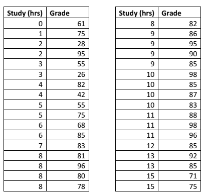
The explanatory variable (X) is:
Study (hours)
The response variable (Y) is:
Grade
Scatterplot

We see a positive correlation. In fact, .
This means that there is a weak, positive correlation between hours studied and exam grade.
What does r2 tell us?
About 29% of exam grade is explained by how many hours you study.
Portions of information contained in this publication/book are printed with permission of Minitab, LLC. All such material remains the exclusive property and copyright of Minitab, LLC. All rights reserved.
Suppose you are given :
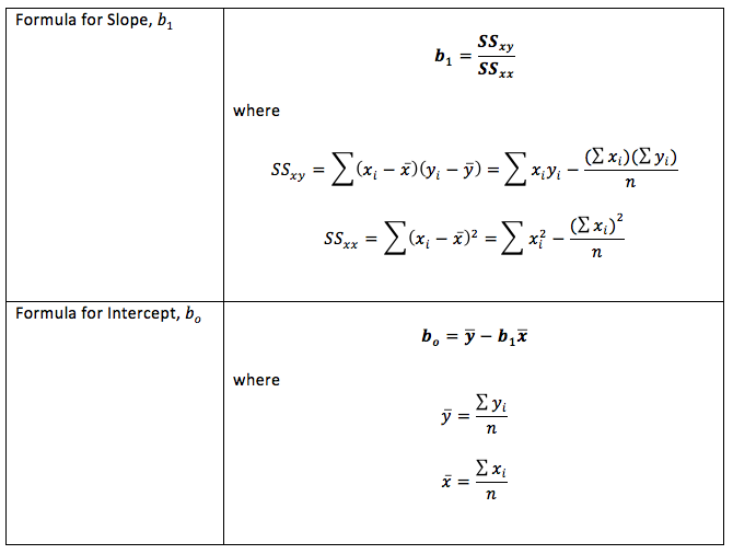
Step 1: Find the slope
Step 2: Find the intercept
Step 3: Show the full linear equation
Using the data set below, determine the correlation, slope, and intercept of the least squares regression line.

= 60 = 4.8
= 38.08 = 2.59
0:00 / 0:00
Solving for the Regression Line (Least Squares Method)

Given a bunch of data coordinates (X,Y), we can generate a scatterplot. Then, we determine the best-fit line to represent the relationship between two quantitative variables: the explanatory variable and the response variable .
The slope , tells us how much changes for every one unit increase in .
Let’s prove this using calculus:
“A unit increase in will change by .”
Wize Concept
The slope and correlation coefficient always have the same sign!
The intercept , tells us the value of when . It is the point where the line crosses the y-axis.
0:00 / 0:00
Example: Solving for the Regression Line (Sxy, Sxx Method)
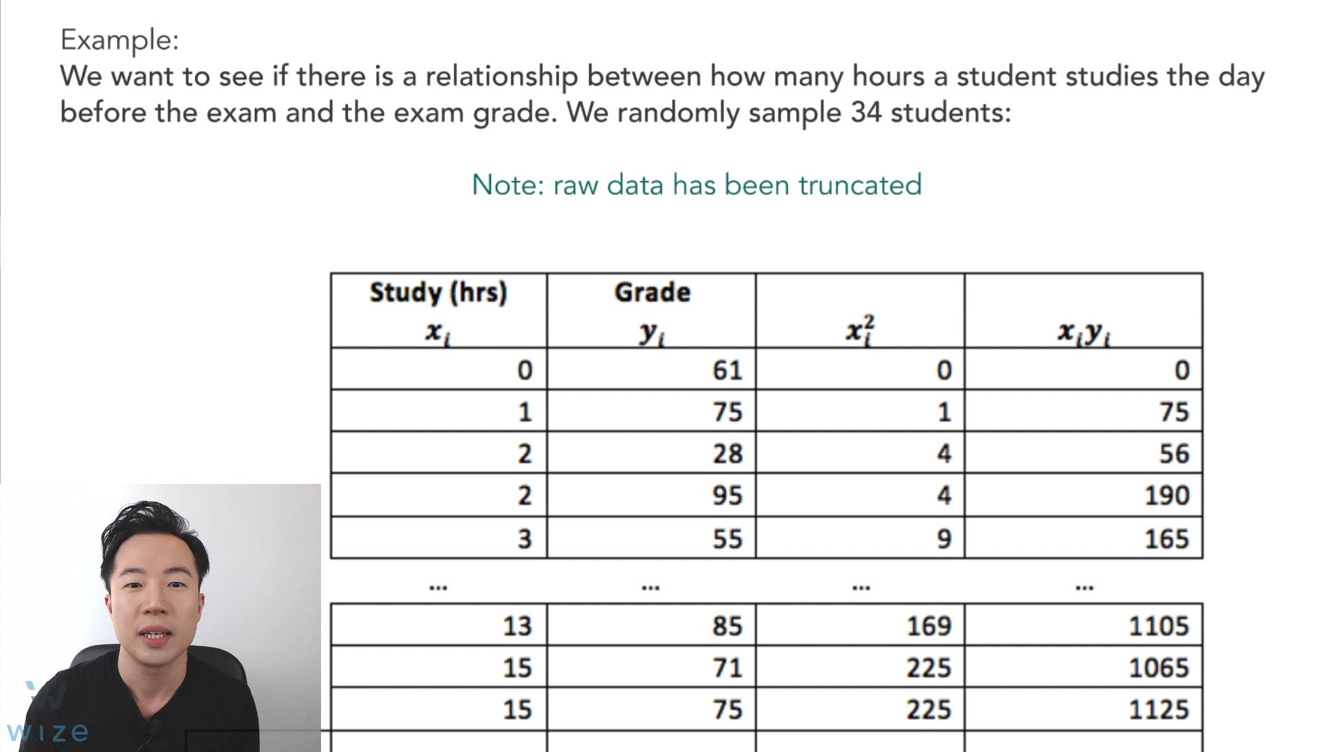
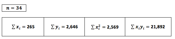
We want to see if there is a relationship between the number of hours a student studies the day before the exam () and the exam grade (). We randomly sample 34 students:
Note: raw data has been truncated
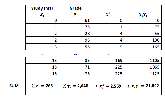
Important:
Scatterplot
Portions of information contained in this publication/book are printed with permission of Minitab, LLC. All such material remains the exclusive property and copyright of Minitab, LLC. All rights reserved.
Step 1: Find the slope
Therefore:
Step 2: Find the intercept
Therefore:
Step 3: Show the full linear equation
Using the information provided below, solve for the slope and intercept of the linear regression equation.
Click on 'HINT' if you are stuck!