Wize University Linear Algebra Textbook > Eigenvalues and Eigenvectors (Spectral Theory)
Eigenvalues and Eigenvectors
Popular Courses
MATH 211
University of Calgary
Linear Algebra
University Study Guides
MATH 133
McGill University
MATH 1ZC3
McMaster University
MATH 152
University of British Columbia
MATH 1600A/B
Western University
Linear Algebra
General Course
MATH 204
Concordia University
MAT188H1
University of Toronto
MATH 125
University of Alberta
NMM 1411A/B
Western University
Linear Algebra
University Study Guides
SC/MATH 1025 3.00
York University
APSC 174
Queen's University
MTH 141
Toronto Metropolitan University
MATH 102
University of Alberta
MATH 115
University of Waterloo
MAT133Y1
University of Toronto
MATH 1B03
McMaster University
MAT223H1
University of Toronto

0:00 / 0:00
Eigenvalues and Eigenvectors
Let be a square matrix. We say that is an eigenvector of with associated eigenvalue if:
Wize Concept
Idea: the eigenvectors of are the vectors that only get stretched by a factor of when multiplied by .
Characteristic Polynomial
The characteristic polynomial of matrix is a degree polynomial defined to be:
The roots of the characteristic polynomial are the eigenvalues of . These are the values of such that .
An eigenvalue's algebraic multiplicity is the number of times it appears as a root (the exponent).
Example
The characteristic polynomial has two roots:
- , with algebraic multiplicity 1 since the factor has an exponent of 1
- , with algebraic multiplicity 2 since the factor has an exponent of 2
How to Find Eigenvalues
Given a square matrix , set the characteristic polynomial equal to and solve for :
Wize Concept
If , we can always find non-trivial solution vectors to the equation .
How to Find Eigenvectors
For each , we find the associated eigenvectors by finding all solutions to the linear system:
Wize Concept
This system has infinitely many solutions because was chosen so that .
The number of basic solutions to the system is the geometric multiplicity of .
We may use Gauss-Jordan elimination to solve the system of linear equations, but we can often solve by inspection!
Shortcut for Matrices
Given a matrix and an eigenvalue , we can find eigenvalues easily by inspection:
0:00 / 0:00
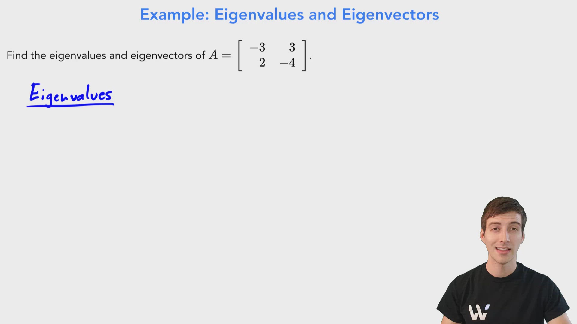
Example: Eigenvalues and Eigenvectors
Find the eigenvalues and eigenvectors of .
Find the Eigenvalues
We solve the equation:
Then the eigenvalues are and . Note that each eigenvalue has algebraic multiplicity 1.
Find the Eigenvectors
Case 1:
We solve the linear system: .
The augmented matrix of this system is:
From here we find that the solution is any vector of the form:
So an eigenvector associated with is:
Case 2:
We solve the linear system:
The augmented matrix of this system is:
From here we find that the solution is any vector of the form:
We prefer not to have fractions, so choosing gives us the basic eigenvector:
Let's check our work:
Practice: Eigenvalues and Eigenvectors
Find all eigenvalues and eigenvectors of the matrix .
State the eigenvalues of in ascending order, along with their algebraic multiplicity.
Practice: Eigenvalues and Eigenvectors
Determine which of the following vectors are eigenvectors of .
[Select all that apply]