Popular Courses
STAT 151
University of Alberta
Statistics
General Course
Intro to Statistics
University Study Guides
STA 100
University of California - Davis
STATS 2244
Western University
STAT 200
University of British Columbia
Intro to Statistics
University Study Guides
STATS 2035
Western University
STAT 161
University of Alberta
QMS 210
Toronto Metropolitan University
STAT 263
Queen's University
STAT 2040
University of Guelph
STAT 251
University of British Columbia
STATS 2B03
McMaster University
STAT 217
University of Calgary
MGTSC 212
University of Alberta
STAT 1060
Dalhousie University
STAT 2060
University of Guelph
BIOL 243
Queen's University
PSYC 204
McGill University

0:00 / 0:00
One-Way ANOVA

By now, you are pros with one-sample hypothesis testing and two-sample hypothesis testing!
Surely, we can compare three or more means! One-way analysis of variance (ANOVA) allows us to determine if there is statistical significance in the difference in means among several groups or samples.
Assumptions for One-way ANOVA
- Each sample is drawn from its respective populations that are assumed to be normal.
- The samples are randomly selected.
- The samples are independent from one another.
- The population variances (and standard deviations) are equal.
- The factor is a categorical variable, but the data they contain (response) must be quantitative.
Example #1:
- Factor: Method of learning (classroom, online, self-study)
- Response: Exam grade
Example #2:
- Factor: Type of fertilizer (synthetic, organic, blend)
- Response: Crop yield
Comparing Several Group Means
Let number of groups being compared (a.k.a. different samples or different populations).
(all population means are equal)
Example
groups
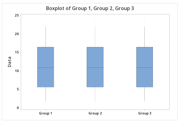
at least one is different than the others
Example

You can also say...
at least two means are not equal such that
In the example above, is statistically significantly different than the other means ( and ). Alternatively, you can say that and .
Portions of information contained in this publication/book are printed with permission of Minitab, LLC. All such material remains the exclusive property and copyright of Minitab, LLC. All rights reserved.

0:00 / 0:00
One-Way ANOVA Table
We can use the one-way ANOVA table to compare multiple population means and determine whether they are all the equal or if they differ.
ANOVA tests result in the following output table:
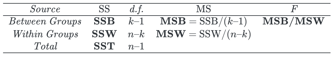
- number of groups (or different samples or populations)
- overall sample size (i.e. the sum of all the observations in all the groups)
Example:
- Group 1 has observations
- Group 2 has observations
- Group 3 has observations
- Thus, the overall sample size
SSB (also called SSC or SSR)
- The sum of squares between groups is the variation in results that exists between groups.
- Logically, we would expect any variation between the groups to be due to the different treatment they received because of the assumption that all else being equal, these different samples all come from populations with the same variance.
- where is the number of different samples or populations.
- is customarily called
SSW (also called SSE)
- The sum of squares within groups is the variation in results that exists within the groups themselves.
- This variation is the result of randomness since within groups individuals all received the same treatment and were selected from the same population.
- where is the overall sample size and is the number of groups
- is customarily called
SST
- The total sum of squares combining the SSB and SSW.
- It encompasses all existing variation in the one-way ANOVA test.
- where is the overall sample size.
MSB (also called MSC or MSR)
- This is the mean of squares between groups.
MSW (also called MSE)
- This is the mean of squares within groups.
Wize Tip
Note that MSW is equal to the overall variance of the sample, and is equal to the overall standard deviation of the sample.
F stat
- One-Way ANOVA F statistic is the ratio between the MSB and MSW:
- The F-test compares the variation between the groups (MSB) to the variation within the group (MSW):
- If the treatments have no impact on the observations, we would expect the variation between and within groups to be the same (resulting in being approximately equal to 1).
- If there is a difference in between and within group variation, it must be as a result of the different treatments which would result in a higher F-score, leading us to conclude that the population means differ.

0:00 / 0:00
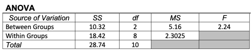
Example: One-way ANOVA Table
Suppose you have a sample of 11 athletes that were randomly split into 3 groups, where members of each group follow different nutrition programs (categorical factors). At the end of the program we can measure how much weight in pounds each athlete has gained (quantitative response).
- This is a one-way ANOVA type of question because we are comparing the average weight gain across the three samples (after the athletes were assigned into 3 groups).
- The variance of the populations can be reasonably expected to be the same since all athletes originate from the same original sample.
Results:

Complete the One-way ANOVA table:

Refer to this helpful table:
Solve for the SSB (also called SSC or SSR), the sum of squares between groups:
- SSB measures the variation in results that exists between groups.
- Any variation between the groups to be due to the different treatment they received.
- where is the number of different samples or populations.
Solve for the SSW (also called SSE), the sum of squares within groups:
- SSW measures the variation in results that exists within the groups themselves.
- This variation is the result of randomness since within groups individuals all received the same treatment and were selected from the same population.
- where is the overall sample size and is the number of different samples or populations.
Solve for the SST, the total sum of squares combining the SSB and SSW:
- where is the overall sample size.
Solve for the MSB (also called MSC or MSR), the mean of squares between groups:
Solve for the MSW (also called MSE), the mean of squares within groups:
Solve for the F-stat:
Practice: One-way ANOVA Table
Rick has 10 Pikamons: 3 grass-types, 4 fire-types, and 3 water-types. Complete the ANOVA table below.
- Provide all answers with at least 2 decimal places (df may be whole number).
- Click on 'HINT' for all the formulas.
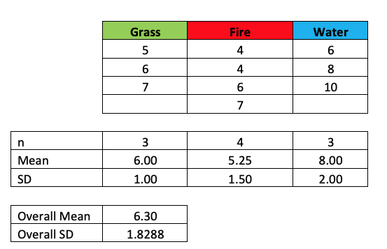
Refer to this helpful table:
| Source of Variation | SS | df | MS | F |
| Between Groups (Factor) | ||||
| Within Groups (Error) | ||||
| Total |