Wize University Linear Algebra Textbook > Vectors

Vector Operations and Linear Combinations

0:00 / 0:00

Vector Operations
There are two main operations we perform on vectors:
Scalar multiplication
Vector addition
Scalar Multiplication
For any scalar kkk, scalar multiplication of a vector v⃗∈Rn\vec{v} \in \reals^nv∈Rn is defined as:

 kv⃗ = k[v1v2⋮vn] = [kv1kv2⋮kvn]∈Rn\boxed{\quad
k\vec{v}
\ =\ 
k
\begin{bmatrix}
  v_1\\ v_2\\ \vdots\\ v_n\\
\end{bmatrix}
\ =\ 
\begin{bmatrix}
  kv_1\\ kv_2\\ \vdots\\ kv_n\\
\end{bmatrix}
\quad} \in \reals^nkv = k​v1​v2​⋮vn​​​ = ​kv1​kv2​⋮kvn​​​​∈Rn 

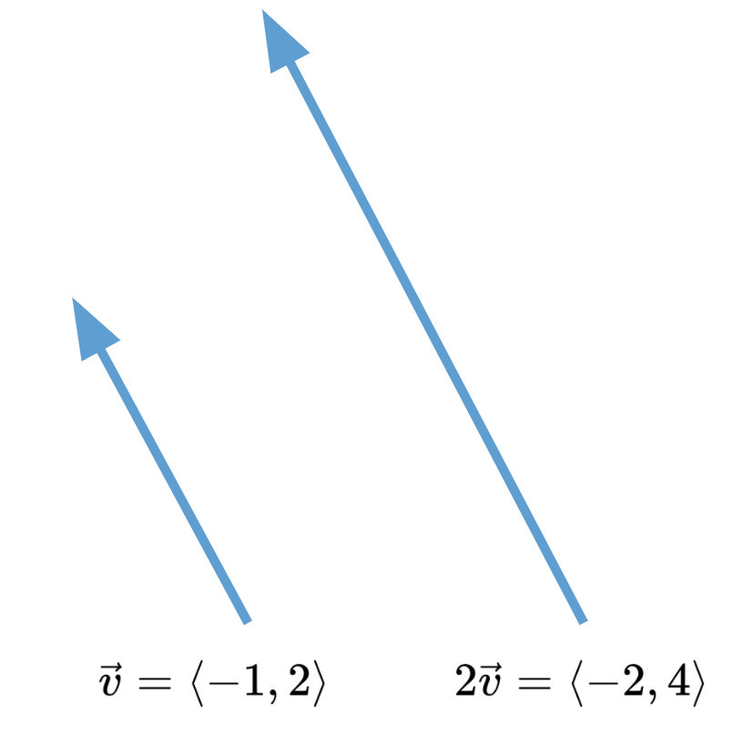
Geometrically, this is represented by stretching (or shrinking) the vector v⃗\vec vv by a factor of kkk without changing its direction.

Below we see that 2v⃗2\vec v2v is twice as long as v⃗\vec vv while still pointing in the same direction:



PAGE BREAK
Collinear Vectors
Vectors v⃗\vec{v}v and u⃗\vec{u}u are collinear or parallel if there is a scalar kkk such that kv⃗=u⃗k\vec{v}=\vec{u}kv=u.



PAGE BREAK
Opposite Vectors
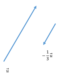
u⃗\vec{u}u and v⃗\vec{v}v point in opposite directions if one vector is a negative scalar multiple of the other.
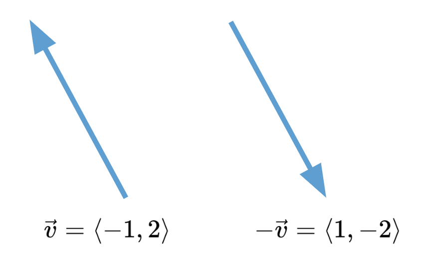
 Here we see that −13u⃗-\frac{1}{3}\vec u−31​u points in the opposite direction of u⃗\vec uu since we multiplied by a negative number:


Negative Vectors
−v⃗=−1v⃗-\vec{v}=-1\vec v−v=−1v is the negative of v⃗\vec{v}v: it has the same length as v⃗\vec vv, but points in the opposite direction.


PAGE BREAK
Vector Addition
For any two vectors u⃗=⟨u1,  u2,  …,  un⟩∈Rn\vec{u}=\lang u_1,\; u_2,\;\dots,\;u_n\rang \in \reals^nu=⟨u1​,u2​,…,un​⟩∈Rn and v⃗=⟨v1,  v2,  …,  vn⟩∈Rn\vec{v}=\lang v_1,\; v_2,\; \dots,\; v_n\rang \in \reals^nv=⟨v1​,v2​,…,vn​⟩∈Rn, vector addition is defined as:

u⃗+v⃗ = [u1u2⋮un]+[v1v2⋮vn] = [u1+v1u2+v2⋮un+vn]∈Rn\boxed{\quad
\vec{u}+\vec{v}
\ =\ 
\begin{bmatrix}
  u_1\\ u_2\\ \vdots\\ u_n\\
\end{bmatrix}
+
\begin{bmatrix}
  v_1\\ v_2\\ \vdots\\ v_n\\
\end{bmatrix}
\ =\ 
\begin{bmatrix}
  u_1+v_1\\ u_2+v_2\\ \vdots\\ u_n+v_n\\
\end{bmatrix}
\quad} \in \reals^nu+v = ​u1​u2​⋮un​​​+​v1​v2​⋮vn​​​ = ​u1​+v1​u2​+v2​⋮un​+vn​​​​∈Rn

Watch Out!
Vectors must be in the same space to add them! E.g. A vector in R2\reals^2R2 cannot be added to a vector in R3\reals^3R3.

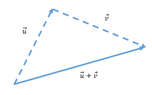
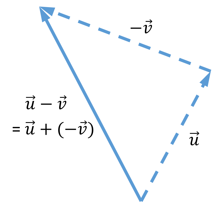
Geometrically,  u⃗+v⃗\vec{u}+\vec{v}u+v works by moving v⃗\vec{v}v so that its tail is at the tip (arrowhead) of u⃗\vec{u}u:


Vector subtraction is based on addition. It is defined as:

u⃗−v⃗=u⃗+(−v⃗)\boxed{\quad
\vec{u}-\vec{v}=\vec{u}+\left(-\vec{v}\right)
\quad}u−v=u+(−v)​



PAGE BREAK
Vector Between Two Points
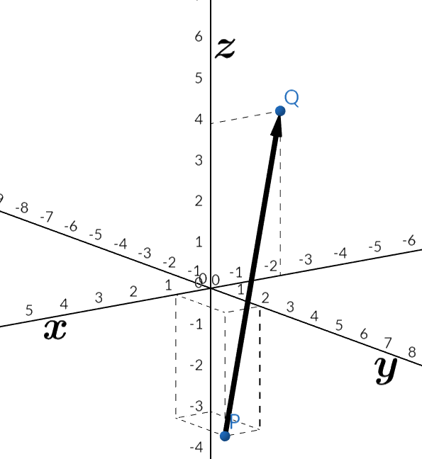
The vector that starts at point PPP and ends at point QQQ is given by:
PQ→=Q⃗−P⃗\boxed{\quad
\overrightarrow{PQ}=\vec Q- \vec P
\quad}PQ​=Q​−P​

Wize Concept
Here we are using the position vectors of points PPP and QQQ, denoted P⃗\vec PP and Q⃗\vec QQ​.
Recall that position vectors are used to treat points as vectors that start at the origin and end at the corresponding point.


Example
Given the points P(1,2,−3)P(1,2,-3)P(1,2,−3) and Q(−2,0,4)Q(-2,0,4)Q(−2,0,4), find the position vector PQ→\overrightarrow{PQ}PQ​.

PQ→=Q⃗−P⃗=[−204]−[12−3]=[−2−10−24−(−3)]=[−3−27]\begin{aligned}
\overrightarrow{PQ}
&= \vec{Q} - \vec{P}\\
&=
\begin{bmatrix}
  -2\\0\\4
\end{bmatrix}
-
\begin{bmatrix}
  1\\2\\-3
\end{bmatrix}\\
&=
\begin{bmatrix}
  -2-1\\0-2\\4-(-3)
\end{bmatrix}\\
&=
\begin{bmatrix}
  -3\\-2\\7
\end{bmatrix}
\end{aligned}PQ​​=Q​−P=​−204​​−​12−3​​=​−2−10−24−(−3)​​=​−3−27​​​

PAGE BREAK
Linear Combinations
Let u⃗, v⃗∈Rn\vec{u}, \ \vec{v} \in \reals^nu, v∈Rn be vectors and let a, b∈Ra, \ b \in \realsa, b∈R be scalars.
A linear combination of u⃗\vec{u}u and v⃗\vec{v}v can be written:
au⃗+bv⃗\boxed{\quad a\vec{u}+b\vec{v}\quad}au+bv​

The result is also a vector in Rn\reals^nRn.

0:00 / 0:00

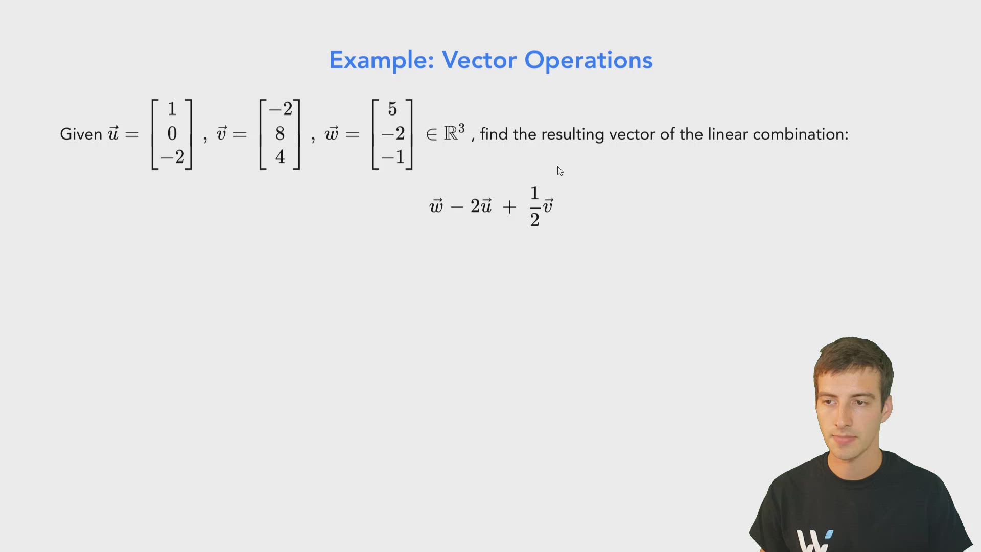
Example: Vector Operations
Given u⃗=[10−2], v⃗=[−284], w⃗=[5−2−1]∈R3\vec{u}=
\begin{bmatrix}
  1\\ 0\\ -2\\
\end{bmatrix}
, \ 
\vec{v}=
\begin{bmatrix}
  -2\\ 8\\ 4\\
\end{bmatrix}
, \ 
\vec{w} =
\begin{bmatrix}
  5\\ -2\\ -1\\
\end{bmatrix} \in \reals^3
u=​10−2​​, v=​−284​​, w=​5−2−1​​∈R3 , find the resulting vector of the linear combination:
w⃗  −  2u⃗  +  12v⃗\vec{w}\;−\;2\vec{u}\;+\;\frac{1}{2}\vec{v}w−2u+21​v

w⃗ − 2u⃗ + 12v⃗ =[5−2−1]−2[10−2]+12[−284]=[5−2−1]−[2×12×02×(−2)]+[12×(−2)12×812×4]=[5−2−1]−[20−4]+[−142]=[5−2+(−1)−2−0+4−1−(−4)+2]=[225]\begin{aligned}
\vec{w} \ −\ 2\vec{u} \ +\ \frac{1}{2}\vec{v}
\ &=
\begin{bmatrix}
  5\\ -2\\ -1\\
\end{bmatrix}
−\colorOne{2}
\begin{bmatrix}
  1\\ 0\\ -2\\
\end{bmatrix}
+\colorTwo{\frac{1}{2}} 
\begin{bmatrix}
  -2\\ 8\\ 4\\
\end{bmatrix}\\
&=
\begin{bmatrix}
  5\\ -2\\ -1\\
\end{bmatrix}
-
\begin{bmatrix}
  \colorOne{2}\times1\\ \colorOne{2}\times0\\ \colorOne{2}\times(-2)\\
\end{bmatrix}
+
\begin{bmatrix}
  \colorTwo{\frac{1}{2}}\times(-2)\\ \colorTwo{\frac{1}{2}}\times8\\ \colorTwo{\frac{1}{2}}\times4\\
\end{bmatrix}\\
&=
\begin{bmatrix}
  5\\ -2\\ -1\\
\end{bmatrix}
-
\begin{bmatrix}
  2\\ 0\\ -4\\
\end{bmatrix}
+
\begin{bmatrix}
  -1\\ 4\\ 2\\
\end{bmatrix}\\
&=
\begin{bmatrix}
  5-2+(-1)\\ -2-0+4\\ -1-(-4)+2\\
\end{bmatrix}\\
&=
\boxed{
\begin{bmatrix}
  2\\ 2\\ 5\\
\end{bmatrix}}
\end{aligned}w − 2u + 21​v ​=​5−2−1​​−2​10−2​​+21​​−284​​=​5−2−1​​−​2×12×02×(−2)​​+​21​×(−2)21​×821​×4​​=​5−2−1​​−​20−4​​+​−142​​=​5−2+(−1)−2−0+4−1−(−4)+2​​=​225​​​​

0:00 / 0:00

Example: Vector Operations
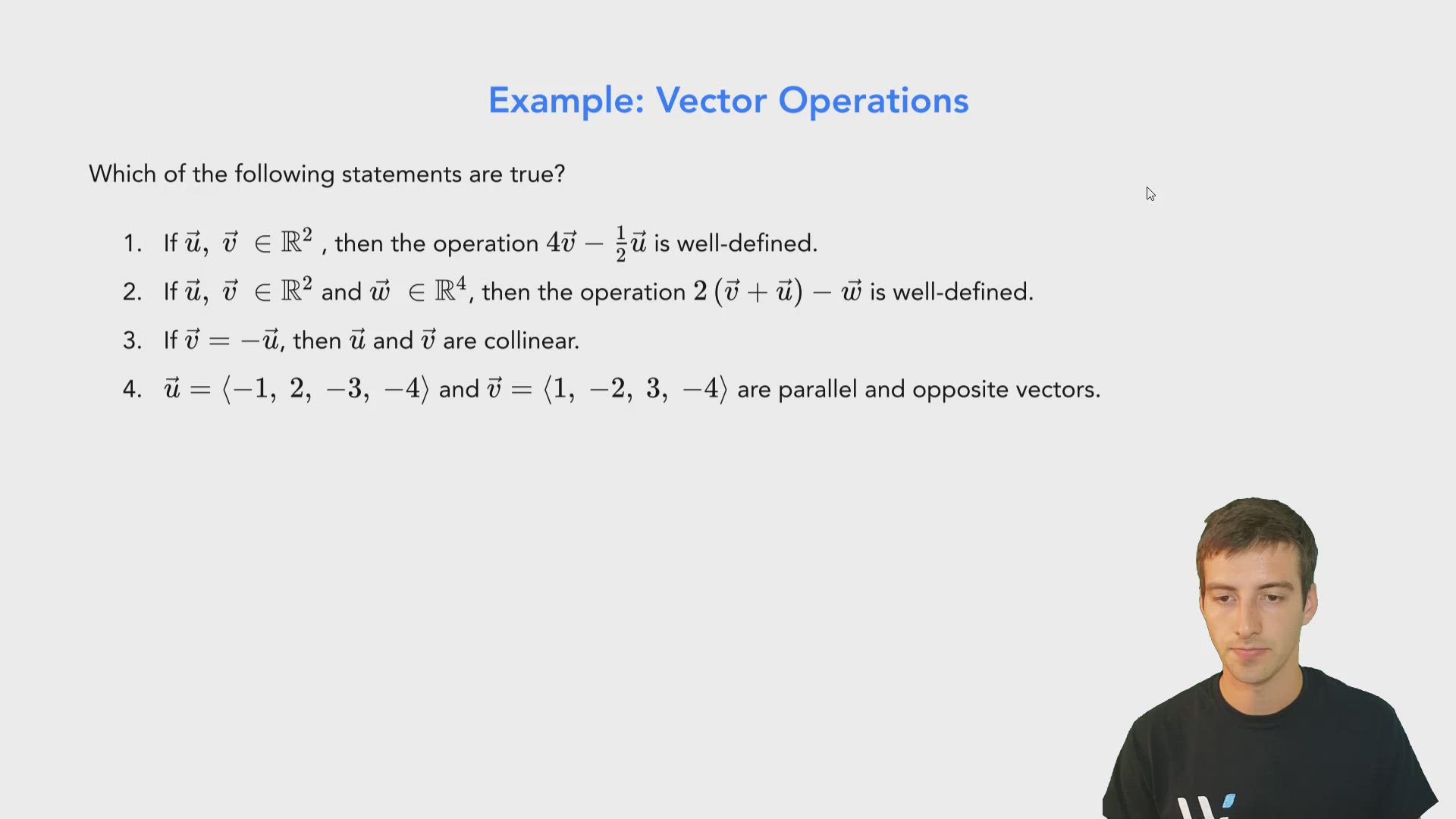
Which of the following statements are true?
If u⃗, v⃗ ∈R2\vec{u},\ \vec{v}\ \in \mathbb{R}^2u, v ∈R2 , then the operation 4v⃗−12u⃗4\vec{v}-\frac{1}{2}\vec{u}4v−21​u is well-defined.
If u⃗, v⃗ ∈R2\vec{u},\ \vec{v}\ \in \mathbb{R}^2u, v ∈R2 and w⃗ ∈R4\vec{w}\ \in \mathbb{R}^4w ∈R4, then the operation 2(v⃗+u⃗)−w⃗2\left(\vec{v}+\vec{u}\right)-\vec{w}2(v+u)−w is well-defined.
If v⃗=−u⃗\vec{v}=-\vec{u}v=−u, then u⃗\vec{u}u and v⃗\vec{v}v are collinear.
u⃗=⟨−1, 2, −3, −4⟩\vec{u}=\lang-1,\ 2,\ -3,\ -4\rangu=⟨−1, 2, −3, −4⟩ and v⃗=⟨1, −2, 3, −4⟩\vec{v}=\lang1,\ -2,\ 3,\ -4\rangv=⟨1, −2, 3, −4⟩ are parallel and opposite vectors.

TRUE: Scalar multiplication is always valid. Since the two vectors are in the same space, R2\mathbb{R}^2R2, vector addition/subtraction is also well-defined.

FALSE: Vector addition/subtraction between vectors in different spaces is never valid.

TRUE: If one vector is the negative of another vector, that means they are a scalar multiples of one another (factor k=−1k=-1k=−1), hence they are collinear.

FALSE: The first three components are indeed scalar multiples of one another (by a factor of -1); however, the last component fails to follow this rule. The vectors are therefore not scalar multiples of one another, thus they are neither parallel nor opposite vectors.

0:00 / 0:00

Example: Vector Operations
P(1,1)P(1,1)P(1,1),  Q(−3,5)Q(-3,5)Q(−3,5), and  R(x,y)R(x,y)R(x,y)  are points in R2\mathbb{R}^2R2, and QR→=−12QP→\overrightarrow{QR}=-\frac{1}{2}\overrightarrow{QP}QR​=−21​QP​.
Find the coordinates of the point R(x,y)R(x,y)R(x,y).

Since we know both PPP and QQQ:
QP→=[1−(−3)1−5]=[4−4]\overrightarrow{QP}=
\begin{bmatrix}
  1-(-3)\\ 1-5\\
\end{bmatrix}=
\begin{bmatrix}
  4\\ -4\\
\end{bmatrix}QP​=[1−(−3)1−5​]=[4−4​]

Now we can use the relationship between QR→\overrightarrow{QR}QR​ and QP→\overrightarrow{QP}QP​:
QR→=−12QP→=−12[4−4]=[−22]\overrightarrow{QR}
=-\frac{1}{2}\overrightarrow{QP}
=-\frac{1}{2}
\begin{bmatrix}
  4\\ -4\\
\end{bmatrix}
=\boxed{\begin{bmatrix}
  -2\\ 2\\
\end{bmatrix}}QR​=−21​QP​=−21​[4−4​]=[−22​]​

And by the formula for a vector between two points, we can also write:

QR→=[x−(−3)y−5]=[x+3y−5]\overrightarrow{QR}
=\begin{bmatrix}
  x-(-3)\\ y-5\\
\end{bmatrix}
=\boxed{
\begin{bmatrix}
  x+3\\ y-5\\
\end{bmatrix}}QR​=[x−(−3)y−5​]=[x+3y−5​]​

The boxed expressions are both representations of QR→\overrightarrow{QR}QR​ so they must be equal:
[x+3y−5]=[−22]\begin{bmatrix}
  \colorOne{x+3}\\ \colorTwo{y-5}\\
\end{bmatrix}
=
\begin{bmatrix}
  \colorOne{-2}\\  \colorTwo{2}\\
\end{bmatrix}[x+3y−5​]=[−22​]

This gives us two equations (one for each component):

x+3=−2  ⟹  x=−5\colorOne{x+3=-2} \quad\implies\quad x=-5x+3=−2⟹x=−5

y−5=2     ⟹  y=7\colorTwo{y-5=2} \ \ \ \quad\implies\quad y=7y−5=2   ⟹y=7

∴  R(−5,7)\therefore\ \ \boxed{R(-5,7)}∴  R(−5,7)​

Practice: Collinear Vectors
Find the value of ccc such that the vectors u⃗=⟨−3,c,3⟩\vec u = \lang −3,c,3 \rangu=⟨−3,c,3⟩ and v⃗=⟨1,−2,−1⟩\vec v = \lang 1,−2,−1 \rangv=⟨1,−2,−1⟩ are collinear.

c=

I don't know

Practice: Collinear Vectors
Given  u⃗=⟨2,−5,6⟩,  v⃗=⟨−4,10,−12⟩,\vec{u}=\lang 2,−5,6\rang ,\ \ \vec{v}=\lang−4,10,−12\rang ,u=⟨2,−5,6⟩,  v=⟨−4,10,−12⟩, and  𝑤⃗=⟨−2,5,−6⟩𝑤⃗=\lang −2,5,−6 \rangw⃗=⟨−2,5,−6⟩, select all statements that are true.

A)  𝑢⃗𝑢⃗u⃗ and 𝑤⃗𝑤⃗w⃗ are collinear

B)  𝑢⃗𝑢⃗u⃗ and 𝑣⃗\vec𝑣v are in opposite directions

C)  v⃗\vec vv is the negative of u⃗\vec uu

D)  𝑢⃗𝑢⃗u⃗ and 𝑤⃗𝑤⃗w⃗ are in opposite directions

I don't know

Practice: Vector Operations
A parallelogram has sides ABABAB, BCBCBC, CDCDCD and DADADA.

The following coordinates are known: A(2,0,1)A(2,0,1)A(2,0,1), C(6,0,0)C(6,0,0)C(6,0,0), and M(3,1,0)M(3,1,0)M(3,1,0), where MMM is the midpoint between AAA and BBB.

Find the vector BD→\overrightarrow{BD}BD.

(4,2,−1)(4,2,-1)(4,2,−1)

(4,−2,2)(4,-2,2)(4,−2,2)

⟨0,−4,3⟩\lang 0,-4,3 \rang⟨0,−4,3⟩

⟨0,3,−4⟩\lang 0,3,-4 \rang⟨0,3,−4⟩

I don't know

Extra Practice

Practice Question

Is the vector (π,e,1)(\pi, e, 1)(π,e,1) in the linear span of  (1,2,3),(−1,0,1)(1, 2, 3), (-1, 0, 1)(1,2,3),(−1,0,1) and  (5,1,−2)(5, 1, -2)(5,1,−2) of  R3\mathbb{R}^3R3 ? Demonstrate a linear combination that does this.

Find the value of h so that (1,-6,4,h) is a linear combination of (1,-2,1,-4), (0,-4,-1,3) and (0,0,2,5).

Linearly independent vectors

Is this set of vectors {[1 3], [2,-2]} linearly independent?   Write [4,-2] as  a linear combination of this set.

Practice: Linear Combination

Show that if u⃗∈Rn\vec u \in \mathbb{R}^nu∈Rn is a linear combination of x⃗,y⃗∈Rn\vec x,\vec y \in \mathbb{R}^nx,y​∈Rn and v⃗∈Rn\vec v \in \mathbb{R}^nv∈Rn is a (different) linear combination of the same  x⃗,y⃗\vec x,\vec yx,y​ then every linear combination  au⃗+bv⃗a\vec u+b\vec vau+bv  for a,b∈Ra,b\in\mathbb{R}a,b∈R is also a linear combination of x⃗,y⃗\vec x,\vec yx,y​ .

133 - FML 3 - 18.1W e.g. 23

Give a mathematical expression that mean v⃗\bcb{\vec{v}}v and w⃗\bcb{\vec{w}}w are parallel.

Practice: Vector Operations

Practice: Vector Operations
If u⃗=[1, 0, −1]\vec{u}=\left[1,\ 0,\ -1\right]u=[1, 0, −1], v⃗=[−2, 4, 1]\vec{v}=\left[-2,\ 4,\ 1\right]v=[−2, 4, 1], and w⃗=[3, 9, −12]\vec{w}=\left[3,\ 9,\ -12\right]w=[3, 9, −12], determine 5u⃗−12v⃗+23w⃗5\vec{u}-\frac{1}{2}\vec{v}+\frac{2}{3}\vec{w}5u−21​v+32​w.

Vector Operations

Practice: Collinear Vectors
Find the value of ccc such that the vectors u⃗=⟨−3,c,3⟩\vec u = \lang −3,c,3 \rangu=⟨−3,c,3⟩ and v⃗=⟨1,−2,−1⟩\vec v = \lang 1,−2,−1 \rangv=⟨1,−2,−1⟩ are collinear.

Practice: Vector Operations

Practice: Vector Operations
If u⃗=[1, 0, −1]\vec{u}=\left[1,\ 0,\ -1\right]u=[1, 0, −1], v⃗=[−2, 4, 1]\vec{v}=\left[-2,\ 4,\ 1\right]v=[−2, 4, 1], and w⃗=[3, 9, −12]\vec{w}=\left[3,\ 9,\ -12\right]w=[3, 9, −12], determine 5u⃗−12v⃗+23w⃗5\vec{u}-\frac{1}{2}\vec{v}+\frac{2}{3}\vec{w}5u−21​v+32​w.

Linear combinations

If u⃗=[5−23]\vec{u}=\begin{bmatrix}5\\-2\\3\end{bmatrix}u=​5−23​​is a linear combination of  v⃗=[−2k3]\vec{v}=\begin{bmatrix}-2\\k\\3\end{bmatrix}v=​−2k3​​and w⃗=[32−1]\vec{w}=\begin{bmatrix}3\\2\\-1\end{bmatrix}w=​32−1​​, what is the value of  kkk?

Write 1 Vector as linear combination of others

Write (16,−15,8)(16,-15, 8)(16,−15,8) as a linear combination of  (1,1,1),(1,1,0),(1,0,−1)(1,1,1), (1,1,0),(1,0,-1)(1,1,1),(1,1,0),(1,0,−1), or show that it is not possible to do so.

133 - FML 3 - 18.1W e.g. 49

 Given v⃗=<0, 4, 3>\bcb{\ol{v} = \left< 0,\, 4,\, 3 \right>}v=⟨0,4,3⟩, find a unit vector perpendicular to v⃗\bcb{\vec{v}}v.

133 - FML 3 - 18.1W e.g. 42

 Find a vector parallel to u⃗=<1, −1, 1>\bcb{\vec{u} = \left< 1,\, -1,\, 1\right>}u=⟨1,−1,1⟩. 

133 - FML 3 - 18.1W e.g. 45

Given the points P=(3, 4, −1)\bcb{P = (3,\, 4,\, -1)}P=(3,4,−1) and Q=(−1, 2, 2)\bcb{Q = (-1,\, 2,\, 2)}Q=(−1,2,2), and the vector u⃗=PQ⃗\bcb{\ol{u} = \vec{PQ}}u=PQ​, find a vector parallel but in the opposite direction to u⃗\bcb{\vec{u}}u.

19.4F_Final_Builder_Ch_4.6_Span_Line_From_FAQ_$\tkco{eg}$_$\key{Final}$_Builder_$\tkcth{4.6.}\tkcf{6}$_$\key{|Strc>5.2}$

Describe the set of all linear combinations (sums of constant multiples of) the vectors:
   v⃗=[111]\vv = \colvecth{1}{1}{1}v=​111​​  and  w⃗=[−121]\vw = \colvecth{-1}{2}{1}w=​−121​​. 

Practice Question: When is 1 Vector a Linear Combination of Others (Has a Solution)

Write (6,5,1)(6,5,1)(6,5,1) as a linear combination of (−2,−1,1),(2,9,15),(2,3,3)(-2,-1,1), (2,9,15), (2,3,3)(−2,−1,1),(2,9,15),(2,3,3) , or show that it is not possible to do so.

$\tkct{cut from 19.4F}$ Mid $\tkco{ S}$ | 133 - FML 3 - 18.1W e.g. 49

 Given v⃗=<0, 4, 3>\bcb{\ol{v} = \left< 0,\, 4,\, 3 \right>}v=⟨0,4,3⟩, find a unit vector perpendicular to v⃗\bcb{\vec{v}}v.

Practice Question: When is 1 Vector a Linear Combination of Others

Is it possible to write down u⃗=(1,2,3)\vec{u}=(1,2,3) u=(1,2,3)as a linear combination of v1⃗=(1,0,2),v2⃗=(0,1,2) and v3⃗=(2,1,6)\vec{v_1}=(1,0,2),\vec{v_2}=(0,1,2)\text{ and }\vec{v_3}=(2,1,6)v1​​=(1,0,2),v2​​=(0,1,2) and v3​​=(2,1,6)? If yes write down u⃗\vec{u}uas a linear combination of other vectors. 

$\tkct{cut from 19.4F}$ Mid $\tkco{ S}$ | 133 - FML 3 - 18.1W e.g. 45

Given the points P=(3, 4, −1)\bcb{P = (3,\, 4,\, -1)}P=(3,4,−1) and Q=(−1, 2, 2)\bcb{Q = (-1,\, 2,\, 2)}Q=(−1,2,2), and the vector u⃗=PQ⃗\bcb{\ol{u} = \vec{PQ}}u=PQ​, find a vector parallel but in the opposite direction to u⃗\bcb{\vec{u}}u.

$\tkct{cut from 19.4F}$ Mid $\tkco{ S}$ | 133 - FML 3 - 18.1W e.g. 42

 Find a vector parallel to u⃗=<1, −1, 1>\bcb{\vec{u} = \left< 1,\, -1,\, 1\right>}u=⟨1,−1,1⟩. 

Find the value of h so that (1,-6,4,h) is a linear combination of (1,-2,1,-4), (0,-4,-1,3) and (0,0,2,5).

19.4F_Final_Builder_Ch_4.6_Span_Line_From_FAQ_$\tkco{eg}$_$\key{Final}$_Builder_$\tkcth{4.6.}\tkcf{4}$_$\key{|Strc>5.2}$

Describe the set of all constant multiples of the vector:
  v⃗=[−121]\vv = \colvecth{-1}{2}{1}v=​−121​​. 

19.4F_Final_Builder_Ch_4.6_Span_Line_From_FAQ_$\tkco{eg}$_$\key{Final}$_Builder_$\tkcth{4.6.}\tkcf{2}$_$\key{|Strc>5.2}$

Describe the set of all constant multiples of the vector v⃗=[11]\vv = \colvec{1}{1}v=[11​]. 

Practice: Properties of Vector Operations

Practice: Properties of Vector Operations
If u⃗, v⃗, w⃗ ∈R3\vec{u},\ \vec{v},\ \vec{w}\ \in R^3u, v, w ∈R3, which of the following statements is/are always true?
i) ∣∣v⃗−u⃗∣∣=−∣∣u⃗−v⃗∣∣\left|\left|\vec{v}-\vec{u}\right|\right|=-\left|\left|\vec{u}-\vec{v}\right|\right|∣∣v−u∣∣=−∣∣u−v∣∣

Vector Addition and Scalar Multiplication

Vector Operations

Practice: Collinear Vectors
Find the value of ccc such that the vectors u⃗=⟨−3,c,3⟩\vec u = \lang −3,c,3 \rangu=⟨−3,c,3⟩ and v⃗=⟨1,−2,−1⟩\vec v = \lang 1,−2,−1 \rangv=⟨1,−2,−1⟩ are collinear.

Practice: Vector Operations

Practice: Vector Operations
If u⃗=[1, 0, −1]\vec{u}=\left[1,\ 0,\ -1\right]u=[1, 0, −1], v⃗=[−2, 4, 1]\vec{v}=\left[-2,\ 4,\ 1\right]v=[−2, 4, 1], and w⃗=[3, 9, −12]\vec{w}=\left[3,\ 9,\ -12\right]w=[3, 9, −12], determine 5u⃗−12v⃗+23w⃗5\vec{u}-\frac{1}{2}\vec{v}+\frac{2}{3}\vec{w}5u−21​v+32​w.

Vector Operations

Practice: Collinear Vectors
Given  u⃗=⟨2,−5,6⟩,  v⃗=⟨−4,10,−12⟩,\vec{u}=\lang 2,−5,6\rang ,\ \ \vec{v}=\lang−4,10,−12\rang ,u=⟨2,−5,6⟩,  v=⟨−4,10,−12⟩, and  𝑤⃗=⟨−2,5,−6⟩𝑤⃗=\lang −2,5,−6 \rangw⃗=⟨−2,5,−6⟩, select all statements that are true.

Vector Operations: Linear Combinations

Find all values of kkk such that the vectors u=(−1,2,k,0)\bm{u}=(-1, 2,k,0)u=(−1,2,k,0) and v=(k,−6,6,0)\bm{v}=(k,-6,6,0)v=(k,−6,6,0) are collinear.

Wize University Linear Algebra Textbook > Vectors

Vector Operations and Linear Combinations

Popular Courses

Vector Operations

Scalar Multiplication

Vector Addition

Vector Between Two Points

Linear Combinations

Example: Vector Operations

Example: Vector Operations

Example: Vector Operations

Practice: Collinear Vectors

Practice: Collinear Vectors

Practice: Vector Operations

Extra Practice

Practice Question

Linearly independent vectors

Practice: Linear Combination

133 - FML 3 - 18.1W e.g. 23

Practice: Vector Operations

Vector Operations

Practice: Vector Operations

Linear combinations

Write 1 Vector as linear combination of others

133 - FML 3 - 18.1W e.g. 49

133 - FML 3 - 18.1W e.g. 42

133 - FML 3 - 18.1W e.g. 45

19.4F_Final_Builder_Ch_4.6_Span_Line_From_FAQ_$\tkco{eg}$_$\key{Final}$_Builder_$\tkcth{4.6.}\tkcf{6}$_$\key{|Strc>5.2}$

Practice Question: When is 1 Vector a Linear Combination of Others (Has a Solution)

$\tkct{cut from 19.4F}$ Mid $\tkco{ S}$ | 133 - FML 3 - 18.1W e.g. 49

Practice Question: When is 1 Vector a Linear Combination of Others

$\tkct{cut from 19.4F}$ Mid $\tkco{ S}$ | 133 - FML 3 - 18.1W e.g. 45

$\tkct{cut from 19.4F}$ Mid $\tkco{ S}$ | 133 - FML 3 - 18.1W e.g. 42

19.4F_Final_Builder_Ch_4.6_Span_Line_From_FAQ_$\tkco{eg}$_$\key{Final}$_Builder_$\tkcth{4.6.}\tkcf{4}$_$\key{|Strc>5.2}$

19.4F_Final_Builder_Ch_4.6_Span_Line_From_FAQ_$\tkco{eg}$_$\key{Final}$_Builder_$\tkcth{4.6.}\tkcf{2}$_$\key{|Strc>5.2}$

Practice: Properties of Vector Operations

Vector Addition and Scalar Multiplication

Vector Operations

Practice: Vector Operations

Vector Operations

Vector Operations: Linear Combinations