0:00 / 0:00

Solutions of a Linear System

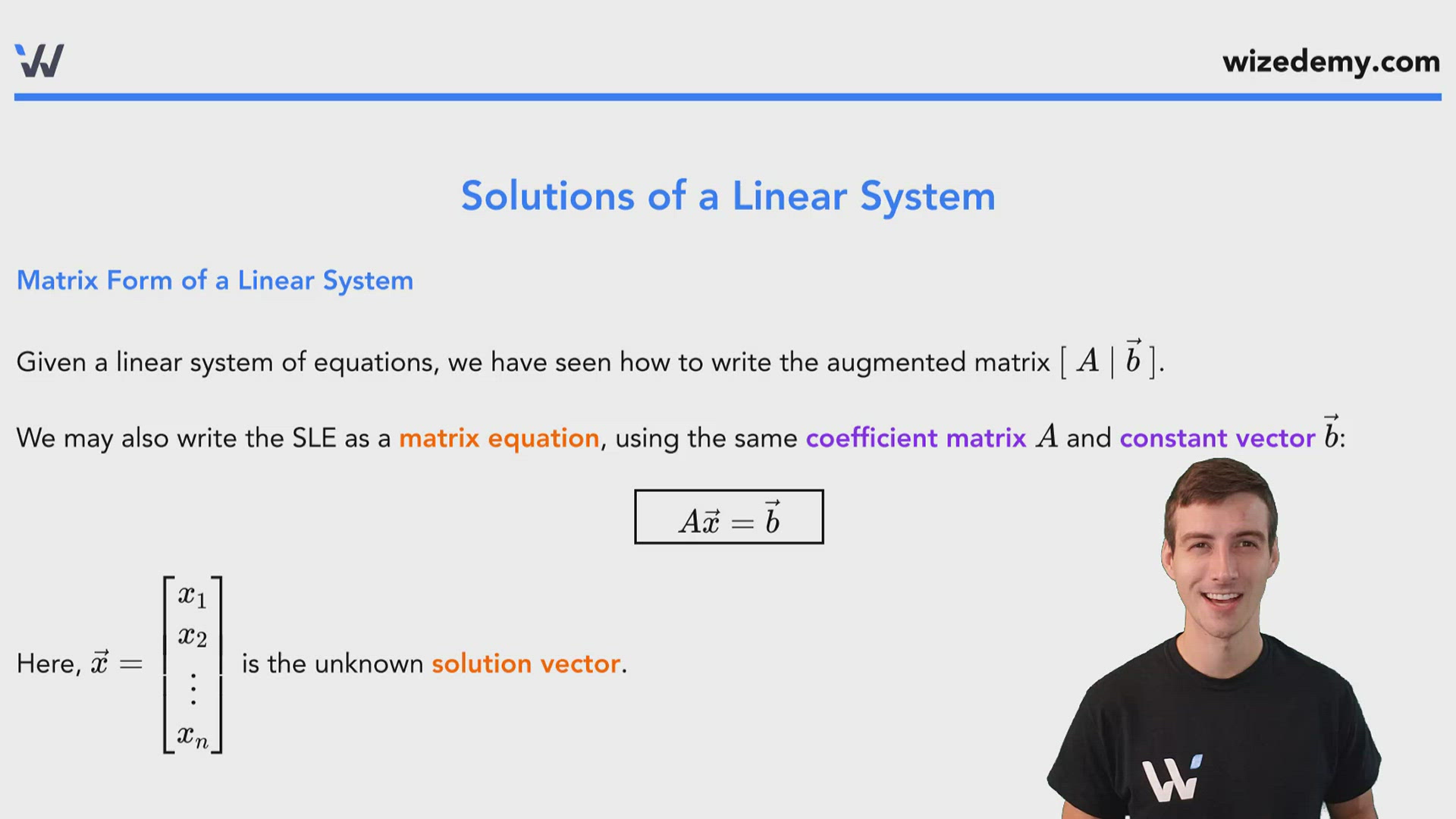
Matrix Form of a Linear System

Given a linear system of equations, we have seen how to write the augmented matrix [ A  b ][\ A\ |\ \vec b\ ].
We may also write the SLE as a matrix equation, using the same coefficient matrix AA and constant vector b\vec b:
Ax=b\boxed{\quad A\vec x = \vec b \quad}
Here, x=[x1x2xn]\vec x = \begin{bmatrix} x_1\\ x_2\\ \vdots\\ x_n \end{bmatrix} is the unknown solution vector.
PAGE BREAK

Procedure to Solve Ax=b\colorOne{A\vec x = \vec b}

  1. Write the linear system as an augmented matrix
  2. Turn the matrix into RREF using EROs
  3. Find all solutions
  4. Use rank to determine the number of solutions
  5. Turn the augmented matrix back into a system of linear equations (assign parameters if needed)
  6. Solve for any missing variables
Example 1
Find the general solution to the system represented by the augmented matrix:
[100a010b001c]\left[\begin{array}{rrr|r} 1&0&0&a\\[0.25em] 0&1&0&b\\[0.25em] 0&0&1&c \end{array}\right]
    {x1=ax2=bx3=c    x=[abc]\begin{aligned} &\implies \begin{cases} x_1=a\\[0.25em] x_2=b\\[0.25em] x_3=c \end{cases}\\[3em] &\implies \boxed{ \vec x = \left[ \begin{array}{l} a\\[0.25em] b\\[0.25em] c \end{array} \right] } \end{aligned}
PAGE BREAK
Example 2
Find the general solution to the system represented by the augmented matrix:
[102a013b]\left[\begin{array}{rrr|r} 1&0&2&a\\[0.25em] 0&1&3&b \end{array}\right]
nrank(A) = 32 = 1n - {\rm rank}(A) \ =\ 3-2 \ =\ 1 free variable.
Note thatx1x_1 and x2x_2 have leading 1s in their columns, but x3x_3 does not.
    x3\implies x_3 is a free variable, and we assign it a parameter: let x3=t\colorOne{x_3=t}.
[102a013b]    {x1+2x3=ax2+3x3=bx3=t    {x1+2t=ax2+3t=bx3=t    {x1=a2tx2=b3tx3=t    x=[a2tb3tt]    x=[ab0]+t[231]   is the 1-parameter family of solutions\begin{aligned} \left[\begin{array}{rrr|r} 1&0&2&a\\[0.25em] 0&1&3&b \end{array}\right] &\implies \left\{\begin{array}{l} x_1+2 \colorOne{x_3}=a\\[0.25em] x_2+3 \colorOne{x_3}=b\\[0.25em] \colorOne{x_3 = t} \end{array}\right.\\[2em] &\implies \left\{\begin{array}{l} x_1+2 \colorOne{t}=a\\[0.25em] x_2+3 \colorOne{t}=b\\[0.25em] \colorOne{x_3 = t} \end{array}\right.\\[2em] &\implies \left\{\begin{array}{l} x_1=a-2 \colorOne{t}\\[0.25em] x_2=b-3 \colorOne{t}\\[0.25em] \colorOne{x_3 = t} \end{array}\right.\\[2em] &\implies \vec x = \left[ \begin{array}{c} a-2 \colorOne{t}\\[0.25em] b-3 \colorOne{t}\\[0.25em] \colorOne{t} \end{array} \right]\\[2em] &\implies \boxed{ \vec x = \left[ \begin{array}{c} a\\ b\\ 0 \end{array} \right] +\colorOne{t} \left[ \begin{array}{c} -2\\ -3\\ 1 \end{array} \right]} \ \ \text{ is the 1-parameter family of solutions} \end{aligned}
0:00 / 0:00

Homogeneous Linear Systems

A system of linear equations is said to be homogeneous if the augmented column is all 0s:
[a11a12a1n0a21a22a2n0am1am2amn0]\left[ \begin{array}{cccc|c} a_{11} & a_{12} & \dots & a_{1n} & \colorThree{0}\\ a_{21} & a_{22} & \dots & a_{2n} & \colorThree{0}\\ \vdots & \vdots &&\vdots&\vdots\\ a_{m1} & a_{m2} & \dots & a_{mn} & \colorThree{0}\\ \end{array} \right]
As a matrix equation, a homogeneous system is written:
Ax=0\boxed{\quad A\vec x = \vec 0 \quad}
Notes
  • A homogeneous system of equations is always consistent!
  • unique solution \rightarrow trivial solution (x=0\vec x = \vec 0)
  • infinitely many solutions
  • The general solution is a linear combination of basic solutions (vectors that appear next to parameters)
Example
[1101000120]\left[\begin{array}{rrrr|r} 1&1&0&1&0\\[0.25em] 0&0&1&2&0 \end{array}\right] represents a system with general solution:
x=s[1100]basic solution+t[1021]basic solution\vec x = s \underbrace{ \begin{bmatrix} -1\\ 1\\ 0\\ 0\\ \end{bmatrix} }_{\text{basic solution}} + t \underbrace{ \begin{bmatrix} -1\\ 0\\ -2\\ 1\\ \end{bmatrix} }_{\text{basic solution}}
The vectors being multiplied by parameters are non-unique basic solutions.
Wize Concept
Any linear combination of basic solutions is another basic solution.

0:00 / 0:00

Example: Solving a Linear System (Unique Solution)

Solve the system of linear equations:
2x+2y2z=2x+2z7=03y=72z\begin{array}{ccccccl} 2x&+&2y&-&2z&=&2\\ x&+&2z&-&7&=&0\\ &&&&3y &=&-7-2z \end{array}
Steps
  1. Let's first write this in augmented matrix form:
2x+2y2z=21x+0y+2z=70x+3y+2z=7[222210270327]\begin{array}{rcr} 2x+2y-2z&=&2\\[0.2em] 1x+0y+2z&=&7\\[0.2em] 0x+3y+2z&=&-7 \end{array} \quad \rightarrow \quad \left[\begin{array}{rrr|r} 2&2&-2&2\\ 1&0&2&7\\ 0&3&2&-7 \end{array}\right]
  1. Turn the matrix into RREF using EROs:
[222210270327]R1R2[102722220327]R22R1[1027026120327]12R2[102701360327]R33R2[10270136001111]111R3[102701360011]R12R3R2+3R3[100501030011]\begin{aligned} &\left[ \begin{array}{rrr|r} 2 & 2 & -2 & 2 \\ 1 & 0 & 2 & 7\\ 0 & 3 & 2 & -7 \\ \end{array} \right] \begin{array}{l} R_1 \leftrightarrow R_2\\ \\ \\ \end{array}\\[2.5em] \longrightarrow &\left[ \begin{array}{rrr|r} 1 & 0 & 2 & 7\\ 2 & 2 & -2 & 2 \\ 0 & 3 & 2 & -7 \\ \end{array} \right] \begin{array}{l} \\ R_2 - 2R_1\\ \\ \end{array}\\[2.5em] \longrightarrow &\left[ \begin{array}{rrr|r} 1 & 0 & 2 & 7\\ 0 & 2 & -6 & -12 \\ 0 & 3 & 2 & -7 \\ \end{array} \right] \begin{array}{l} \\ \dfrac{1}{2}R_2\\ \\ \end{array}\\[2.5em] \longrightarrow &\left[ \begin{array}{rrr|r} 1 & 0 & 2 & 7\\ 0 & 1 & -3 & -6 \\ 0 & 3 & 2 & -7 \\ \end{array} \right] \begin{array}{l} \\ \\ R_3 - 3R_2\\ \end{array}\\[2.5em] \longrightarrow &\left[ \begin{array}{rrr|r} 1 & 0 & 2 & 7\\ 0 & 1 & -3 & -6 \\ 0 & 0 & 11 & 11 \\ \end{array} \right] \begin{array}{l} \\ \\ \dfrac{1}{11}R_3\\ \end{array}\\[2.5em] \longrightarrow &\left[ \begin{array}{rrr|r} 1 & 0 & 2 & 7\\ 0 & 1 & -3 & -6 \\ 0 & 0 & 1 & 1 \\ \end{array} \right] \begin{array}{l} R_1 - 2 R_3\\ R_2 + 3 R_3\\ \\ \end{array}\\[2.5em] \longrightarrow &\left[ \begin{array}{rrr|r} 1 & 0 & 0 & 5\\ 0 & 1 & 0 & -3 \\ 0 & 0 & 1 & 1 \\ \end{array} \right] \end{aligned}
  1. Find all solutions to the SLE:
The coefficient matrix has 3 leading 1s and 3 columns: rank(A)=n{\rm rank}(A) = n     \implies there is a unique solution.
Rewrite the augmented matrix back into a system of linear equations:
x=5y=3z=1\begin{array}{c} x&=&5\\ y&=&-3\\ z&=&1 \end{array}
Therefore, the unique solution is
x=[531]\boxed{\vec x = \begin{bmatrix} 5\\ −3\\ 1 \end{bmatrix}}
0:00 / 0:00

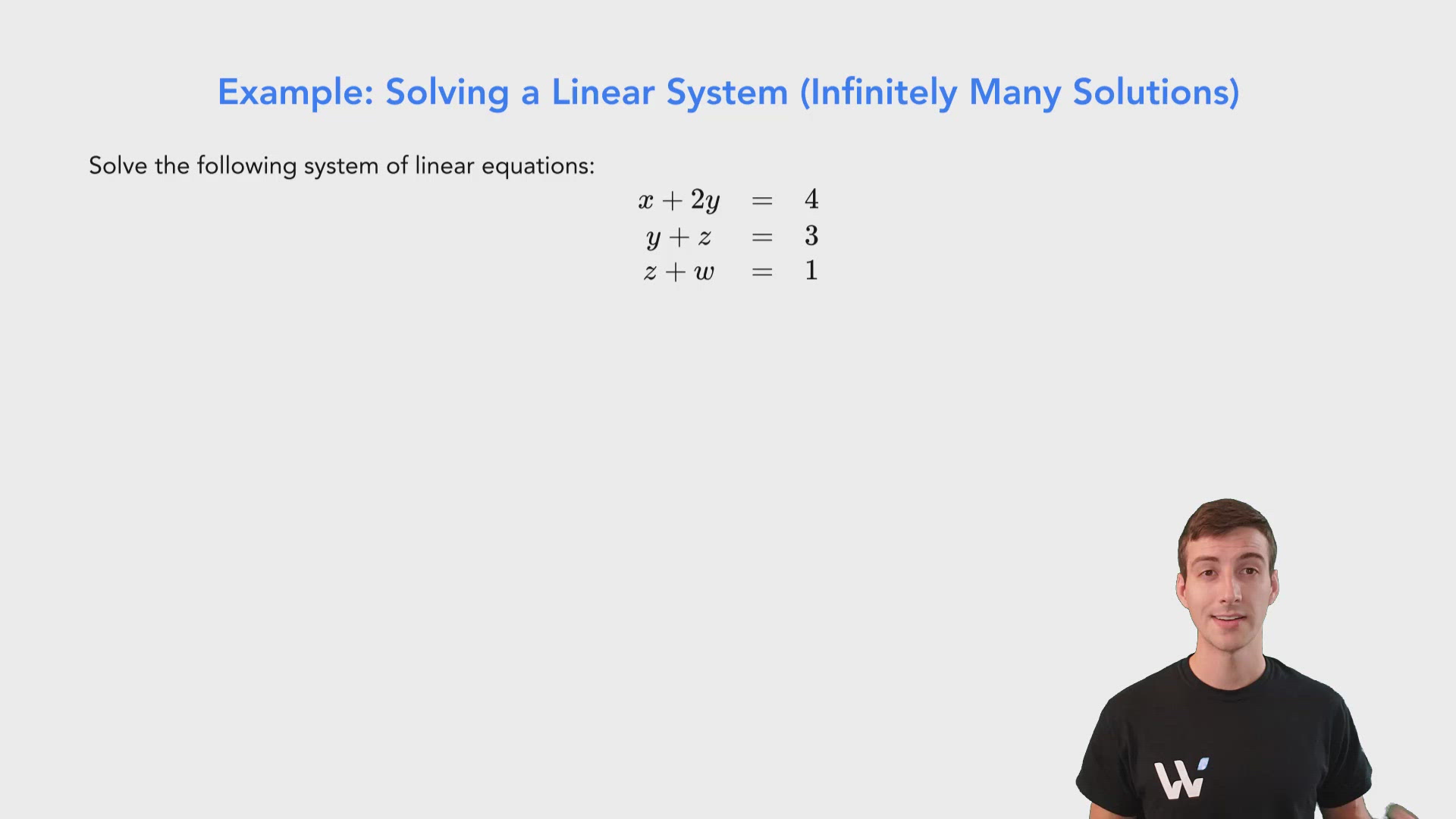
Example: Solving a Linear System (Infinitely Many Solutions)

Solve the following system of linear equations:
x+2y=4y+z=3z+w=1\begin{array}{c} x+2y&=&4\\ y+z&=&3\\ z+w&=&1 \end{array}
The standard form of the linear system is 1x+2y+0z+0w=40x+1y+1z+0w=30x+0y+1z+1w=1\begin{array}{c} 1x+2y+0z+0w&=&4\\ 0x+1y+1z+0w&=&3\\ 0x+0y+1z+1w&=&1 \end{array} and the augmented matrix is [120040110300111]\left[\begin{array}{rrrr|r} 1&2&0&0&4\\ 0&1&1&0&3\\ 0&0&1&1&1 \end{array} \right].
(Note that the order of the variables does not matter, but be consistent!)
We need to reduce the matrix to RREF:
[120040110300111]R12R2[102020110300111]R1+2R3R2R3[100200101200111]\begin{aligned} &\left[ \begin{array}{rrrr|r} 1 & 2 & 0 & 0 & 4\\ 0 & 1 & 1 & 0 & 3\\ 0 & 0 & 1 & 1 & 1\\ \end{array} \right] \begin{array}{l} R_1 - 2R_2\\ \\ \\ \end{array}\\[2.5em] \longrightarrow &\left[ \begin{array}{rrrr|r} 1 & 0 & -2 & 0 & -2\\ 0 & 1 & 1 & 0 & 3\\ 0 & 0 & 1 & 1 & 1\\ \end{array} \right] \begin{array}{l} R_1 + 2R_3\\ R_2 - R_3\\ \\ \end{array}\\[2.5em] \longrightarrow &\left[ \begin{array}{rrrr|r} 1 & 0 & 0 & 2 & 0\\ 0 & 1 & 0 & -1 & 2\\ 0 & 0 & 1 & 1 & 1\\ \end{array} \right] \end{aligned}
There are 3 leading 1s and 4 columns in the RREF, so rank(A)=3  <  n=4{\rm rank}(A)=3 \ \ \bm<\ \ n=4, so there are infinitely many solutions.
nrank(A) = 43 = 1n-{\rm rank}(A) \ =\ 4-3 \ =\ 1 so there is one free variable (1-parameter family of solutions).
Let's assign a parameter to the free variable (the column with a missing leading 1, ww) and rewrite the SLE using the RREF.
Let w=t\colorTwo{w=t}. (Remember to include this equation in the list of equations we obtain from the RREF. We need a solution for all variables!)
{x+2w=0yw=2z+w=1w=t    {x+2t=0yt=2z+t=1w=t    {x=2ty=2+tz=1tw=t\begin{cases} x+2\colorTwo{w}&=&0\\ y-\colorTwo{w}&=&2\\ z+\colorTwo{w}&=&1\\ \colorTwo{w}&=&\colorTwo{t} \end{cases} \quad\implies\quad \begin{cases} x+2\colorTwo{t}&=&0\\ y-\colorTwo{t}&=&2\\ z+\colorTwo{t}&=&1\\ \colorTwo{w}&=&\colorTwo{t} \end{cases} \quad\implies\quad \begin{cases} x&=&-2\colorTwo{t}\\ y&=&2+\colorTwo{t}\\ z&=&1-\colorTwo{t}\\ \colorTwo{w}&=&\colorTwo{t} \end{cases}
Therefore, the 1-parameter family of solutions is x=[0210]+t[2111]\boxed{ \vec x = \begin{bmatrix} 0\\ 2\\ 1\\ 0\\ \end{bmatrix} + \colorTwo{t} \begin{bmatrix} -2\\ 1\\ -1\\ 1\\ \end{bmatrix} }.
Solve the following system of linear equations. What type of solution is it?
3x1+6x2=12x1+4x2=2x2+x3=3\begin{aligned} 3x_1 + 6x_2&= 1\\ 2x_1 + 4x_2 &=2\\ x_2 + x_3 &= 3 \end{aligned}

Solve the following homogeneous system of linear equations. What type of solution is it?
2x1x2+2x4=02x2+4x3x4=0\begin{aligned} 2x_1-x_2+2x_4 &= 0\\ 2x_2 + 4x_3 − x_4 &= 0 \end{aligned}